The following movies are simulations of an atomic force microscope (AFM) tip approaching to and retracting from a sample surface.
The potential between the tip and the sample ("sample potential") was chosen to be of the Lennard-Jones type ("6-12 potential"),
Vsample(z) = A z -12 - B z -6,
where z denotes the tip-sample distance and A and B are interaction parameters.
In an AFM, the tip is attached to a flexible cantilever and thus is also exposed to the "cantilever potential",
Vcant(z) = k/2 (z-z0)2,
where k is the spring constant of the cantilever and z0 is the tip-sample distance
for an un-flexed cantilever.
The three movies are for the same tip-sample potential, but for three different spring constants:
Play Movie 1
Movie 1:
Large spring constant (k = 0.5 N/m). No jump-in or jump-out instabilities occur, since the
stiff cantilever can balance the sample forces at all times and thus keeps the tip "in place".
Movie 1:
Large spring constant (k = 0.5 N/m). No jump-in or jump-out instabilities occur, since the
stiff cantilever can balance the sample forces at all times and thus keeps the tip "in place".
View/download as
AVI movie.
Play Movie 2
Movie 2:
Intermediate spring constant (k = 0.05 N/m). Both jump-in and jump-out
instabilities occur, since the cantilever cannot balance the sample force at all times.
Movie 2:
Intermediate spring constant (k = 0.05 N/m). Both jump-in and jump-out
instabilities occur, since the cantilever cannot balance the sample force at all times.
View/download as
AVI movie.
Play Movie 3
Movie 3:
Small spring constant (k = 0.02 N/m). Again, both jump-in and jump-out instabilities occur,
but the jump-out instability is not observed in this movie since the cantilever is so soft that
the tip basically "gets stuck" on the sample surface.
Movie 3:
Small spring constant (k = 0.02 N/m). Again, both jump-in and jump-out instabilities occur,
but the jump-out instability is not observed in this movie since the cantilever is so soft that
the tip basically "gets stuck" on the sample surface.
View/download as
AVI movie.
Further explanations:
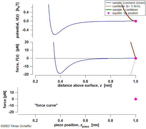
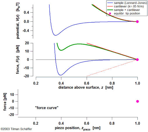
The top graph in each movie shows the sample potential (blue curve), the cantilever potential
(red curve) and the sum of both constituting the total potential (green curve).
The values are plotted vs. the tip-sample distance. The equilibrium position of the tip (pink marker)
is located at a minimum of the total potential.
The middle graph in each movie shows the force exerted onto the tip by the sample,
Fsample (z) = - d/dz Vsample(z), (blue curve), the force exerted
onto the tip by the cantilever, Fcant(z) = - k (z-z0)
(=Hooke's law), (red curve), and the sum of both constituting the total force onto the tip (green curve).
The values are again plotted vs. the tip-sample distance. The equilibrium position of the tip (pink marker)
is located at a zero of the total force. (Note: A simple method for graphically locating the
equilibrium position is finding the intersection of the sample force with the negative cantilever
force (dotted red line).)
The bottom graph in each movie shows the force measured in an AFM
spectroscopy measurement. Such a measurement is called a "force curve", as it records cantilever
force as a function of position above the surface. Typically, this position is not chosen as the
tip-sample distance z but instead as z0, the tip-sample distance for an
un-flexed cantilever. The reason for this is that z0 is directly available in the
AFM since it is the position of the piezoelectric element that moves the cantilever toward and away
from the surface, whereas z needs to be calculated from z0 and
Fsample.
The parameters chosen for these simulations were
A = 10-134 J m12 and B = 10-77 J m6.
This corresponds to a very simple interaction configuration where just one atom from the tip
interacts with just one atom from the sample. The energy in the top graph (potential) is plotted in units of
kBT (Boltzmann constant kB =~ 1.38×10⁻²³ J/K
and T = 298 K =~ 25 °C) (1 kBT =~ 1/40 eV at room temperature).


